

Microsoft Office 2019 is the current version of Microsoft Office, a productivity suite, succeeding Office 2016. It was released to general availability for Windows 10 and for macOS on September 24, 2018.
1.CONCAT
This new function is like CONCATENATE, but better. First of all, it’s shorter and easier to type. But it also supports range references, in addition to cell references. Learn more about CONCAT.
Syntax
CONCAT(text1, [text2],…)
| Argument | Description |
| text1 (required) |
Text item to be joined. A string, or array of strings, such as a range of cells. |
| [text2, …] (optional) |
Additional text items to be joined. There can be a maximum of 253 text arguments for the text items. Each can be a string, or array of strings, such as a range of cells. |
For example, =CONCAT(“The”,” “,”sun”,” “,”will”,” “,”come”,” “,”up”,” “,”tomorrow.”) will return The sun will come up tomorrow.
2.IFS
Tired of typing complicated, nested IF functions? The IFS function is the solution. With this function, conditions are tested in the order that you specify. If passed, the result is returned. You can also specify an else “catch all” if none of the conditions are met. Learn more about IFS.
Simple syntax
- IFS([Something is True1, Value if True1, [Something is True2, Value if True2],…[Something is True127, Value if True127])
Notes:
- The IFS function allows you to test up to 127 different conditions.
- For example:
- Which says IF(A1 equals 1, then display 1, IF A1 equals 2, then display 2, or else if A1 equals 3, then display 3).
- It’s generally not advisable to use too many conditions with IF or IFS statements, as multiple conditions need to be entered in the correct order, and can be very difficult to build, test and update.
- =IFS(A1=1,1,A1=2,2,A1=3,3)
Example 1
 89,”A”,A2>79,”B”,A2>69,”C”,A2>59,”D”,TRUE,”F”)” />
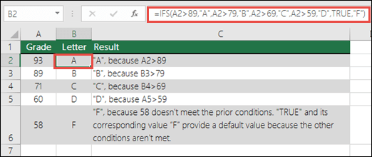
The formula for cells A2:A6 is:
- =IFS(A2>89,”A”,A2>79,”B”,A2>69,”C”,A2>59,”D”,TRUE,”F”)
Which says IF(A2 is Greater Than 89, then return a “A”, IF A2 is Greater Than 79, then return a “B”, and so on and for all other values less than 59, return an “F”).
Example 2
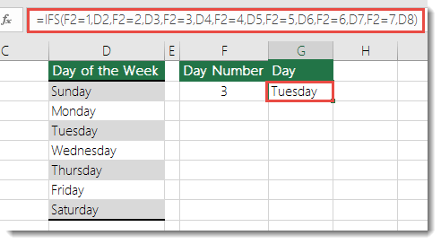
The formula in cell G7 is:
- =IFS(F2=1,D2,F2=2,D3,F2=3,D4,F2=4,D5,F2=5,D6,F2=6,D7,F2=7,D8)
Which says IF(the value in cell F2 equals 1, then return the value in cell D2, IF the value in cell F2 equals 2, then return the value in cell D3, and so on, finally ending with the value in cell D8 if none of the other conditions are met).
3.MAXIFS
This function returns the largest number in a range, that meets a single or multiple criteria. Learn more about MAXIFS.
Syntax
MAXIFS(max_range, criteria_range1, criteria1, [criteria_range2, criteria2], …)
| Argument | Description |
| max_range (required) |
The actual range of cells in which the maximum will be determined. |
| criteria_range1 (required) |
Is the set of cells to evaluate with the criteria. |
| criteria1 (required) |
Is the criteria in the form of a number, expression, or text that defines which cells will be evaluated as maximum. The same set of criteria works for the MINIFS, SUMIFS, and AVERAGEIFS functions. |
|
criteria_range2, |
Additional ranges and their associated criteria. You can enter up to 126 range/criteria pairs. |
Remarks
- The size and shape of the max_range and criteria_rangeN arguments must be the same, otherwise these functions return the #VALUE! error.
Examples
Copy the example data in each of the following tables, and paste it in cell A1 of a new Excel worksheet. For formulas to show results, select them, press F2, and then press Enter. If you need to, you can adjust the column widths to see all the data.
Example 1
| Grade | Weight |
| 89 | 1 |
| 93 | 2 |
| 96 | 2 |
| 85 | 3 |
| 91 | 1 |
| 88 | 1 |
| Formula | Result |
| =MAXIFS(A2:A7,B2:B7,1) | 91
In criteria_range1 the cells B2, B6, and B7 match the criteria of 1. Of the corresponding cells in max_range, A6 has the maximum value. The result is therefore 91. |
4.MINIFS
This function is similar to MAXIFS, but it returns the smallest number in a range, that meets a single or multiple criteria. Learn more about MINIFS.
Syntax
MINIFS(min_range, criteria_range1, criteria1, [criteria_range2, criteria2], …)
| Argument | Description |
| min_range (required) |
The actual range of cells in which the minimum value will be determined. |
| criteria_range1 (required) |
Is the set of cells to evaluate with the criteria. |
| criteria1 (required) |
Is the criteria in the form of a number, expression, or text that defines which cells will be evaluated as minimum. The same set of criteria works for the MAXIFS, SUMIFS and AVERAGEIFS functions. |
| criteria_range2, criteria2, …(optional) |
Additional ranges and their associated criteria. You can enter up to 126 range/criteria pairs. |
Remarks
- The size and shape of the min_range and criteria_rangeN arguments must be the same, otherwise these functions return the #VALUE! error.
Examples
Copy the example data in each of the following tables, and paste it in cell A1 of a new Excel worksheet. For formulas to show results, select them, press F2, and then press Enter. If you need to, you can adjust the column widths to see all the data.
Example 1
| Grade | Weight |
| 89 | 1 |
| 93 | 2 |
| 96 | 2 |
| 85 | 3 |
| 91 | 1 |
| 88 | 1 |
| Formula | Result |
| =MINIFS(A2:A7,B2:B7,1) | 88
In criteria_range1 the cell B2, B6, and B7 match the criteria of 1. Of the corresponding cells in min_range, A7 has the minimum value. The result is therefore 88. |
Example 2
| Weight | Grade |
| 10 | b |
| 11 | a |
| 100 | a |
| 111 | b |
| 1 | a |
| 1 | a |
| Formula | Result |
| =MINIFS(A2:A5,B3:B6,”a”) | 10
Note: The criteria_range and min_range aren’t aligned, but they are the same shape and size. In criteria_range1, the 1st, 2nd, and 4th cells match the criteria of “a.” Of the corresponding cells in min_range, A2 has the minimum value. The result is therefore 10. |
Example 3
| Weight | Grade | Class | Level |
| 10 | b | Business | 100 |
| 11 | a | Technical | 100 |
| 12 | a | Business | 200 |
| 13 | b | Technical | 300 |
| 14 | b | Technical | 300 |
| 15 | b | Business | 400 |
| Formula | Result | ||
| =MINIFS(A2:A7,B2:B7,”b”,D2:D7,”>100″) | 13
In criteria_range1, B2, B5, B6 and B7 match the criteria of “b.” Of the corresponding cells in criteria_range2, D5, D6, and D7 match the criteria of >100. Finally, of the corresponding cells in min_range, D5 has the minimum value. The result is therefore 13. |
Example 4
| Weight | Grade | Class | Level |
| 10 | b | Business | 8 |
| 1 | a | Technical | 8 |
| 100 | a | Business | 8 |
| 11 | b | Technical | 0 |
| 1 | a | Technical | 8 |
| 1 | b | Business | 0 |
| Formula | Result | ||
| =MINIFS(A2:A7,B2:B7,”b”,D2:D7,A8) | 1
The criteria2 argument is A8. However, because A8 is empty, it is treated as 0 (zero). The cells in criteria_range2 that match 0 are D5 and D7. Finally, of the corresponding cells in min_range, A7 has the minimum value. The result is therefore 1. |
5.SWITCH
This function evaluates an expression against a list of values in order, and returns the first matching result. If no results match, the “else” is returned. Learn more about SWITCH.
Overview
In its simplest form, the SWITCH function says:
- =SWITCH(Value to switch, Value to match1…[2-126], Value to return if there’s a match1…[2-126], Value to return if there’s no match)
Where you can evaluate up to 126 matching values and results.
See the following formula:
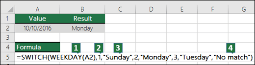
- Value to switch? In this case, WEEKDAY(A2) equals 2.
- What value do you want to match? In this case, it’s 1, 2 and 3.
- If there’s a match, what do you want to return as a result? In this case, it would be Sunday for 1, Monday for 2 and Tuesday for 3.
- Default value to return if there’s no match found. In this case, it’s the text “No match”.
Note: If there are no matching values, and no default argument is supplied, the SWITCH function returns the #N/A! error.
Examples
You can copy the example data in the following table and paste it in cell A1 of a new Excel worksheet to see the SWITCH function in action. If the formulas don’t show results, you can select them, then press F2 > Enter. If you need to, you can adjust the column widths to see all the data.
Example
| Value | Formula | Result |
| 2 | =SWITCH(WEEKDAY(A2),1,”Sunday”,2,”Monday”,3,”Tuesday”,”No match”) | Because A2=2, and Monday is the result argument corresponding to the value 2, SWITCH returns Monday |
| 99 | =SWITCH(A3,1,”Sunday”,2,”Monday”,3,”Tuesday”) |
Because there’s no match and no else argument, SWITCH returns #N/A! |
| 99 | =SWITCH(A4,1,”Sunday”,2,”Monday”,3,”Tuesday”,”No match”) | No match |
| 2 | =SWITCH(A5,1,”Sunday”,7,”Saturday”,”weekday”) | weekday |
| 3 | =SWITCH(A6,1,”Sunday”,2,”Monday”,3,”Tuesday”,”No match”) | Tuesday |
6.TEXTJOIN
This function combines text from multiple ranges, and each item is separated by a delimiter that you specify. Learn more about TEXTJOIN.
Syntax
TEXTJOIN(delimiter, ignore_empty, text1, [text2], …)
| argument | Description |
| delimiter (required) |
A text string, either empty, or one or more characters enclosed by double quotes, or a reference to a valid text string. If a number is supplied, it will be treated as text. |
| ignore_empty (required) |
If TRUE, ignores empty cells. |
| text1 (required) |
Text item to be joined. A text string, or array of strings, such as a range of cells. |
| [text2, …] (optional) |
Additional text items to be joined. There can be a maximum of 252 text arguments for the text items, including text1. Each can be a text string, or array of strings, such as a range of cells. |
For example, =TEXTJOIN(” “,TRUE, “The”, “sun”, “will”, “come”, “up”, “tomorrow.”) will return The sun will come up tomorrow.
Remarks
- If the resulting string exceeds 32767 characters (cell limit), TEXTJOIN returns the #VALUE! error.
Examples
Copy the example data in each of the following tables, and paste it in cell A1 of a new Excel worksheet. For formulas to show results, select them, press F2, and then press Enter. If you need to, you can adjust the column widths to see all the data.
Example 1
| Currency | |
| US Dollar | |
| Australian Dollar | |
| Chinese Yuan | |
| Hong Kong Dollar | |
| Israeli Shekel | |
| South Korean Won | |
| Russian Ruble | |
| Formula: | =TEXTJOIN(“, “, TRUE, A2:A8) |
| Result: | US Dollar, Australian Dollar, Chinese Yuan, Hong Kong Dollar, Israeli Shekel, South Korean Won, Russian Ruble |
Example 2
| A’s | B’s |
| a1 | b1 |
| a2 | b2 |
| a4 | b4 |
| a5 | b5 |
| a6 | b6 |
| a7 | b7 |
| Formula: | =TEXTJOIN(“, “, TRUE, A2:B8) |
| Result: | a1, b1, a2, b2, a4, b4, a5, b5, a6, b6, a7, b7
If ignore_empty=FALSE, the result would be: a1, b1, a2, b2, , , a4, b4, a5, b5, a6, b6, a7, b7 |
Example 3
| City | State | Postcode | Country |
| Tulsa | OK | 74133 | US |
| Seattle | WA | 98109 | US |
| Iselin | NJ | 08830 | US |
| Fort Lauderdale | FL | 33309 | US |
| Tempe | AZ | 85285 | US |
| end | |||
| , | , | , | ; |
| Formula: | =TEXTJOIN(A8:D8, TRUE, A2:D7) | ||
| Result: |
Tulsa,OK,74133,US;Seattle,WA,98109,US;Iselin,NJ,08830,US;Fort Lauderdale,FL,33309,US;Tempe,AZ,85285,US;en |
Step by Step! តក់ៗពេញបំពង់

wow great brother,thanks for your share knowlegd
LikeLiked by 1 person
It’s my pleasure, Somphors.
LikeLike